
ML on the Materials Project, part 2: trees, and overfitting caught
Same data, one change of model, and R2 jumps from 0.095 to 0.637. Plus the train-versus-test gap that shows memorization as a number.
Part 1 ended with an honest floor: linear regression explaining about 10 percent of band gap variation across 26,568 oxides (R2 = 0.095). Part 2 changes nothing but the model, and watches what happens.
Why trees
A decision tree is twenty-questions played with data. Training grows a flowchart of yes/no threshold questions (“is the electronegativity spread above 1.8?”), each chosen because it best separates high-gap from low-gap materials, repeated inside every branch. A new material walks the flowchart and takes the number at its leaf.
The key property: a question asked only inside one branch expresses this feature matters differently depending on that one, an interaction. A straight line must give every feature one fixed effect everywhere; a tree’s rules are contextual by construction. Chemistry is contextual too. That is the whole bet.
The catch, and two cures
An unlimited tree memorizes: it grows a branch for every training material and ends up perfect on data it studied, poor on anything new. That is overfitting, and instead of describing it, this experiment includes one unlimited tree specifically to catch it in the act.
The cures are teamwork. A Random Forest trains hundreds of trees, each deliberately handicapped (a random sample of rows, a random subset of features per question), then averages them: each tree overfits in its own random direction, and the directions cancel. Gradient boosting trains shallow trees in sequence, each one fitted to the errors of the ensemble so far, a chain of error-correctors.
The race
Four models, identical features, identical train/test split, so every number is comparable to part 1. For each, both the training score and the test score, because the gap between them is memorization made visible.
| model | train R2 | test R2 | test MAE |
|---|---|---|---|
| linear regression | 0.091 | 0.095 | 1.218 eV |
| single tree, unlimited | 0.904 | 0.452 | 0.686 eV |
| random forest (300 trees) | 0.875 | 0.637 | 0.646 eV |
| gradient boosting | 0.684 | 0.587 | 0.757 eV |
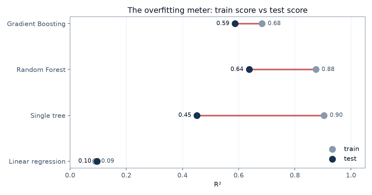
Three readings:
The single tree is the educational star. It scored 0.904 on material it studied and 0.452 on material it had not. That cliff between columns is overfitting, not as a concept but as a number you can point at.
The forest wins. Test R2 0.637, average miss 0.65 eV. Same data, same features, and the explanation went from 10 percent to 64 percent while the typical error halved. The crowd of differently-wrong trees kept the pattern and averaged away the noise.
Boosting lost at defaults, while being the least overfit of the tree models. With tuning it usually wins; tuning was deliberately out of scope, defaults keep the comparison clean.
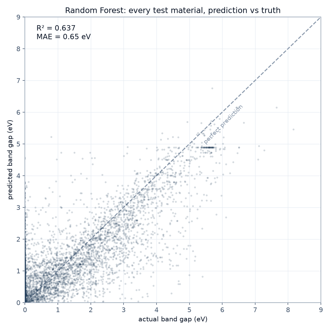
The parity plot shows the improvement directly: part 1’s nearly horizontal cloud now hugs the diagonal. And it contains two details worth finding.
The vertical wall at zero. The metals. Their true gap is exactly 0, but an average of 300 trees almost never says exactly zero, so every metal receives a small phantom gap. Regression is the wrong question for “is this a metal”: that is a yes/no matter, and it is part 3.
A short horizontal streak near predicted 4.9: dozens of materials with different true gaps all receiving one identical prediction. Identical predictions mean identical features, and identical features with different answers means polymorphs. The blind spot planted in part 1 just photographed itself. A useful general rule: horizontal banding in a parity plot means your features are blind to something the truth cares about.
The hidden gem
Why did the unlimited tree score only 0.904 on its own training data, when it was free to memorize everything? Because some of its training questions have contradictory answers: polymorphs share identical features but different gaps, so a leaf holding them must give one number for materials that genuinely differ. Even perfect memorization cannot beat that ceiling. No model on these features can.
The standing caveat
Every number here is still slightly flattered: polymorph twins are scattered across the train and test sets, so the models occasionally sat an exam containing questions they had seen. Part 4 measures that flattery properly, with grouped splits. The 0.637 is the before picture.
The takeaway
Model choice was worth six times the explanation (0.095 to 0.637) and cost nothing but a few seconds of compute. But both of this part’s deeper lessons were about evaluation, not models: read train-versus-test as a memorization meter, and know your data well enough to explain why even the training score has a ceiling.
Part 3: is it even a metal? Classification, the confusion matrix, and why a 97 percent accurate model can be useless.
Found a mistake? Good, tell me. This publication flags its own suspect values. Reach me on LinkedIn.