
ML on the Materials Project, part 1: the honest floor
Fetching 26,568 real oxides, turning formulas into numbers a model can learn from, and why a first score of R2 = 0.095 is a good start.
This is the first part of a series applying machine learning to real Materials Project data, one model family at a time, with every number reported honestly. Part 1 builds the foundation everything else stands on: a dataset, a way to turn formulas into numbers, and a first model whose job is to be humble.
The plan in one sentence
Predict a material’s band gap, the property that separates metals from semiconductors from insulators, from nothing but its chemical composition, and be honest about how well that works.
Step 1: the dataset
Machine learning needs examples. Ours come from the Materials Project API: every oxide (oxygen-containing compound) made of two or three elements. That query returns 26,568 entries, fetched in 27 pages of 1,000.
Before any modeling, three facts about this dataset shape everything downstream:
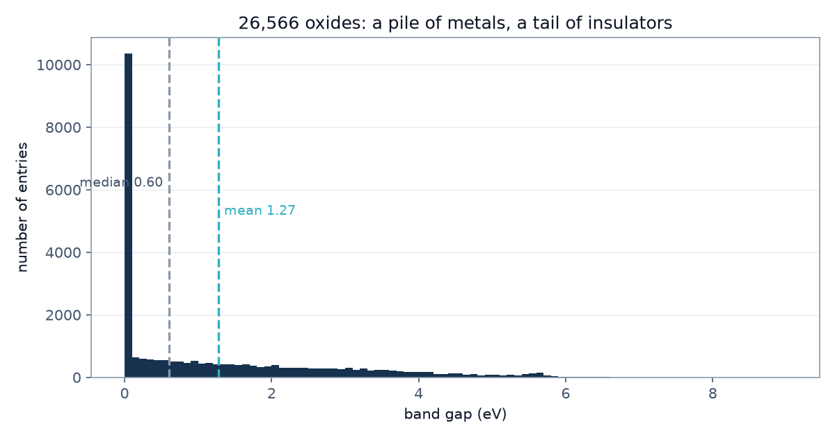
First, the distribution is lopsided: roughly 10,000 entries are metals with a gap of exactly zero, followed by a long thin tail of insulators reaching past 8 eV. That is why the mean (1.27 eV) sits far from the median (0.60 eV), and why “the average material” barely exists here.

Second, a third of the dataset is polymorphs: the same formula appearing as different crystal structures with different properties. SiO2 alone appears 322 times. Remember this; it returns in part 4 as the villain.
Third, only 3,642 of the entries are thermodynamically stable, and 18,903 are theoretical, structures that have never existed outside a computer.
Step 2: formulas into numbers
A model is arithmetic. It cannot read “Fe2O3”. So every composition must become a list of numbers, called features, before learning can happen.
The trick is to describe a compound through the known properties of its elements. Fe2O3 is 40 percent iron, 60 percent oxygen by atom count, so:
mean electronegativity = 0.40 x 1.83 (Fe) + 0.60 x 3.44 (O) = 2.80
spread                 = 3.44 - 1.83 = 1.61
The weighted mean describes the compound’s “average atom”. The spread measures how different the elements are: a large electronegativity spread hints at ionic bonding, which tends to mean wider gaps. One number, real chemistry.
Twelve such features per material (means and spreads of electronegativity, atomic mass, atomic number, and periodic row, plus element count and oxygen fraction), computed by a hand-written featurizer of about a hundred lines. The professional tool for this job is the matminer library, which produces 145 features; building the small version by hand first means none of them are ever a black box.
One honest detail: two materials were skipped because they contain helium, which has no electronegativity. Skipped and reported, never silently filled with a fake value.
And one planted limitation: these features come only from the formula. All 322 SiO2 polymorphs therefore get identical features but have different true gaps. No model in this series can escape that ceiling, and we will measure it properly later.
Step 3: the floor
Before any clever model, two rules. Split the data (80 percent for training, 20 percent held back for honest grading), and establish a baseline: predict the training-set average for everything. The baseline’s R2 is 0.00 by definition; anything real must beat it.
The first real model is linear regression: one learned weight per feature. The result, on the held-out test set:
| model | MAE | R2 |
|---|---|---|
| always guess 1.27 eV | 1.285 eV | 0.00 |
| linear regression | 1.218 eV | 0.095 |
R2 of 0.095 means the model explains about 10 percent of why band gaps differ. Here is what that looks like:
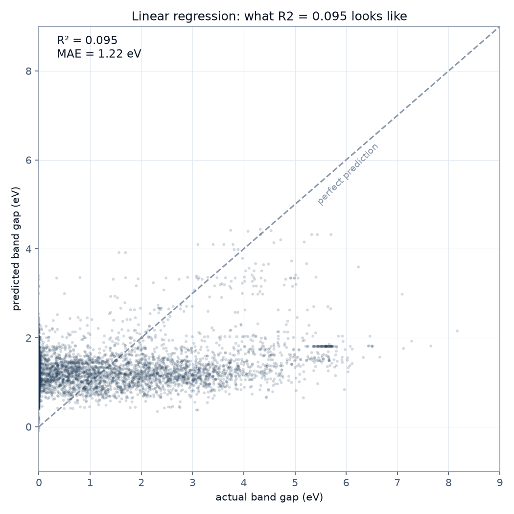
Every dot is one test material: true gap across, prediction up. A perfect model puts every dot on the diagonal. Ours produced a nearly horizontal cloud: it predicts between 0.5 and 2 eV for almost everything, whatever the truth is. R2 = 0.095 does not mean “somewhat wrong”. It means “refusing to commit”.
Why a weak score is a good start
A straight line has to give every feature one fixed effect, everywhere, always. But chemistry is contextual: the effect of electronegativity depends on what else is in the compound, effects saturate, interactions multiply. Band gap chemistry is made of bends, and a linear model cannot bend. The weak score is not a failure of the data; it is a measurement of the mismatch between the model’s shape and the problem’s shape.
That measurement is the point. Every model in the rest of this series now has a floor to beat, and when the next one jumps past 0.095, the jump itself will say exactly what the added complexity bought.
Part 2: tree models, which are built entirely out of bends.
Found a mistake? Good, tell me. This publication flags its own suspect values. Reach me on LinkedIn.